PyBroom Example - Simple¶

This notebook is part of pybroom.

This notebook shows the simplest usage of pybroom when performing a curve fit of a single dataset. Possible applications are only hinted. For a more complex (and interesting!) example using multiple datasets see pybroom-example-multi-datasets.

In [1]:

import numpy as np
from numpy import sqrt, pi, exp, linspace
from lmfit import Model
import matplotlib.pyplot as plt
%matplotlib inline
%config InlineBackend.figure_format='retina'  # for hi-dpi displays

In [2]:

import lmfit
print('lmfit: %s' % lmfit.__version__)

lmfit: 0.9.7

In [3]:

import pybroom as br

Create Noisy Data¶

In [4]:

x = np.linspace(-10, 10, 101)

In [5]:

peak1 = lmfit.models.GaussianModel(prefix='p1_')
peak2 = lmfit.models.GaussianModel(prefix='p2_')
model = peak1 + peak2

In [6]:

params = model.make_params(p1_amplitude=1, p2_amplitude=1,
                           p1_sigma=1, p2_sigma=1)

In [7]:

y_data = model.eval(x=x, p1_center=-1, p2_center=2, p1_sigma=0.5, p2_sigma=1, p1_amplitude=1, p2_amplitude=2)
y_data.shape

Out[7]:

(101,)

In [8]:

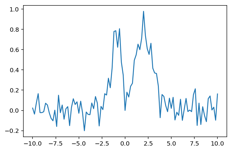
y_data += np.random.randn(*y_data.shape)/10

In [9]:

plt.plot(x, y_data)

Out[9]:

[<matplotlib.lines.Line2D at 0x7f0a072b36d8>]

../_images/notebooks_pybroom-example_11_1.png

Model Fitting¶

In [10]:

params = model.make_params(p1_center=0, p2_center=3,
                           p1_sigma=0.5, p2_sigma=1,
                           p1_amplitude=1, p2_amplitude=2)
result = model.fit(y_data, x=x, params=params)

Fit result from an lmfit Model can be inspected with with fit_report or params.pretty_print():

In [11]:

print(result.fit_report())

[[Model]]
    (Model(gaussian, prefix='p1_') + Model(gaussian, prefix='p2_'))
[[Fit Statistics]]
    # function evals   = 75
    # data points      = 101
    # variables        = 6
    chi-square         = 0.885
    reduced chi-square = 0.009
    Akaike info crit   = -466.467
    Bayesian info crit = -450.776
[[Variables]]
    p1_amplitude:   0.99193692 +/- 0.073905 (7.45%) (init= 1)
    p1_sigma:       0.50403814 +/- 0.043298 (8.59%) (init= 0.5)
    p1_center:     -0.93732080 +/- 0.042639 (4.55%) (init= 0)
    p2_amplitude:   1.80858848 +/- 0.098970 (5.47%) (init= 2)
    p2_sigma:       0.92432008 +/- 0.060121 (6.50%) (init= 1)
    p2_center:      2.04760247 +/- 0.057497 (2.81%) (init= 3)
    p1_fwhm:        1.18691910 +/- 0.101960 (8.59%)  == '2.3548200*p1_sigma'
    p1_height:      0.78511041 +/- 0.055989 (7.13%)  == '0.3989423*p1_amplitude/max(1.e-15, p1_sigma)'
    p2_fwhm:        2.17660743 +/- 0.141575 (6.50%)  == '2.3548200*p2_sigma'
    p2_height:      0.78059804 +/- 0.041815 (5.36%)  == '0.3989423*p2_amplitude/max(1.e-15, p2_sigma)'
[[Correlations]] (unreported correlations are <  0.100)
    C(p1_amplitude, p1_sigma)    =  0.613
    C(p2_amplitude, p2_sigma)    =  0.612
    C(p1_amplitude, p2_sigma)    = -0.263
    C(p1_sigma, p2_sigma)        = -0.251
    C(p1_center, p2_sigma)       = -0.210
    C(p1_amplitude, p2_amplitude)  = -0.194
    C(p1_sigma, p2_amplitude)    = -0.192
    C(p1_center, p2_amplitude)   = -0.154
    C(p1_sigma, p2_center)       =  0.148
    C(p1_amplitude, p2_center)   =  0.139
    C(p1_center, p2_center)      =  0.110

In [12]:

result.params.pretty_print()

Name             Value      Min      Max   Stderr     Vary     Expr Brute_Step
p1_amplitude    0.9919     -inf      inf  0.07391     True     None     None
p1_center      -0.9373     -inf      inf  0.04264     True     None     None
p1_fwhm          1.187     -inf      inf    0.102    False 2.3548200*p1_sigma     None
p1_height       0.7851     -inf      inf  0.05599    False 0.3989423*p1_amplitude/max(1.e-15, p1_sigma)     None
p1_sigma         0.504        0      inf   0.0433     True     None     None
p2_amplitude     1.809     -inf      inf  0.09897     True     None     None
p2_center        2.048     -inf      inf   0.0575     True     None     None
p2_fwhm          2.177     -inf      inf   0.1416    False 2.3548200*p2_sigma     None
p2_height       0.7806     -inf      inf  0.04182    False 0.3989423*p2_amplitude/max(1.e-15, p2_sigma)     None
p2_sigma        0.9243        0      inf  0.06012     True     None     None

These methods a re convenient but extracting the data from the lmfit object requires some work and the knowledge of lmfit object structure.

pybroom comes to help, extracting data from fit results and returning pandas DataFrame in tidy format that can be much more easily manipulated, filtered and plotted.

Glance¶

Glancing at the fit results (dropping some verbose columns):

In [13]:

dg = br.glance(result)
dg.drop('model', 1).drop('message', 1)

Out[13]:

	method	num_params	num_data_points	chisqr	redchi	AIC	BIC	num_func_eval	success
0	leastsq	6	101	0.884993	0.009316	-466.466867	-450.776144	75	True

The glance function returns a DataFrame with one row per fit-result object.

Application Idea¶

If you fit N models to the same dataset you can compare statistics such as reduced-\(\chi^2\)

Or, fitting several with several methods (and datasets) you can study the convergence properties using reduced-\(\chi^2\), number of function evaluation and success rate.

Tidy¶

Tidy fit results for all the parameters:

In [14]:

dt = br.tidy(result)
dt

Out[14]:

	name	value	min	max	vary	expr	stderr	init_value
0	p1_amplitude	0.991937	-inf	inf	True	None	0.073906	1.0
1	p1_center	-0.937321	-inf	inf	True	None	0.042640	0.0
2	p1_fwhm	1.186919	-inf	inf	False	2.3548200*p1_sigma	0.101961	NaN
3	p1_height	0.785110	-inf	inf	False	0.3989423*p1_amplitude/max(1.e-15, p1_sigma)	0.055990	NaN
4	p1_sigma	0.504038	0.000000	inf	True	None	0.043299	0.5
5	p2_amplitude	1.808588	-inf	inf	True	None	0.098970	2.0
6	p2_center	2.047602	-inf	inf	True	None	0.057498	3.0
7	p2_fwhm	2.176607	-inf	inf	False	2.3548200*p2_sigma	0.141575	NaN
8	p2_height	0.780598	-inf	inf	False	0.3989423*p2_amplitude/max(1.e-15, p2_sigma)	0.041815	NaN
9	p2_sigma	0.924320	0.000000	inf	True	None	0.060121	1.0

The tidy function returns one row for each parameter.

In [15]:

dt.loc[dt.name == 'p1_center']

Out[15]:

	name	value	min	max	vary	expr	stderr	init_value
1	p1_center	-0.937321	-inf	inf	True	None	0.04264	0.0

Augment¶

Tidy dataframe with data function of the independent variable (‘x’). Columns include the data being fitted, best fit, best fit components, residuals, etc.

In [16]:

da = br.augment(result)
da.head()

Out[16]:

	x	data	best_fit	residual	Model(gaussian, prefix='p1_')	Model(gaussian, prefix='p2_')
0	-10.0	0.022939	1.005185e-37	-0.022939	4.947068e-71	1.005185e-37
1	-9.8	-0.036681	1.647759e-36	0.036681	5.735959e-68	1.647759e-36
2	-9.6	0.071802	2.577558e-35	-0.071802	5.681800e-65	2.577558e-35
3	-9.4	0.165100	3.847602e-34	-0.165100	4.808258e-62	3.847602e-34
4	-9.2	-0.021899	5.480738e-33	0.021899	3.476253e-59	5.480738e-33

The `augment <>`__ function returns one row for each data point.

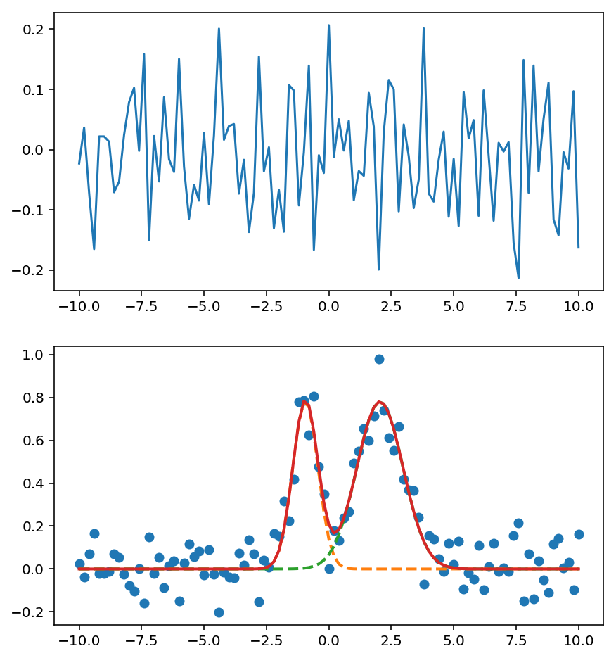
In [17]:

d = br.augment(result)

In [18]:

fig, ax = plt.subplots(2, 1, figsize=(7, 8))
ax[1].plot('x', 'data', data=d, marker='o', ls='None')
ax[1].plot('x', "Model(gaussian, prefix='p1_')", data=d, lw=2, ls='--')
ax[1].plot('x', "Model(gaussian, prefix='p2_')", data=d, lw=2, ls='--')
ax[1].plot('x', 'best_fit', data=d, lw=2)
ax[0].plot('x', 'residual', data=d);

../_images/notebooks_pybroom-example_30_0.png

Application Idea¶

Fitting N datasets with the same model (or N models with the same dataset) you can automatically build a panel plot with seaborn using the dataset (or the model) as categorical variable. This example is illustrated in pybroom-example-multi-datasets.