PyBroom Example - Multiple Datasets - Minimize

This notebook is part of pybroom.

This notebook demonstrate using pybroom when performing Maximum-Likelihood fitting (scalar minimization as opposed to curve fitting) of a set of datasets with lmfit.minimize. We will show that pybroom greatly simplifies comparing, filtering and plotting fit results from multiple datasets. For an example using curve fitting see pybroom-example-multi-datasets.

In [1]:

%matplotlib inline
%config InlineBackend.figure_format='retina'  # for hi-dpi displays
import numpy as np
import pandas as pd
import matplotlib.pyplot as plt
from matplotlib.pylab import normpdf
import seaborn as sns
from lmfit import Model
import lmfit
print('lmfit: %s' % lmfit.__version__)

lmfit: 0.9.5

/home/docs/checkouts/readthedocs.org/user_builds/pybroom/envs/stable/lib/python3.4/site-packages/IPython/html.py:14: ShimWarning: The `IPython.html` package has been deprecated. You should import from `notebook` instead. `IPython.html.widgets` has moved to `ipywidgets`.
  "`IPython.html.widgets` has moved to `ipywidgets`.", ShimWarning)

In [2]:

sns.set_style('whitegrid')

In [3]:

import pybroom as br

Create Noisy Data

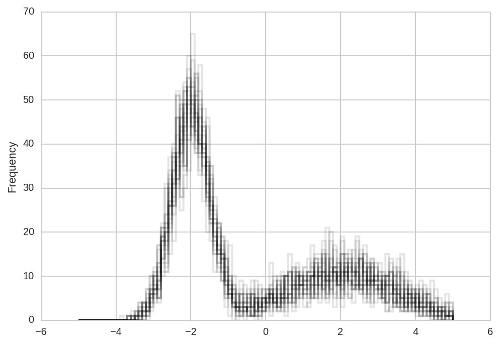
Simulate N datasets which are identical except for the additive noise.

In [4]:

N = 20  # number of datasets
n = 1000  # number of sample in each dataset

np.random.seed(1)
d1 = np.random.randn(20, int(0.6*n))*0.5 - 2
d2 = np.random.randn(20, int(0.4*n))*1.5 + 2
d = np.hstack((d1, d2))

In [5]:

ds = pd.DataFrame(data=d, columns=range(d.shape[1])).stack().reset_index()
ds.columns = ['dataset', 'sample', 'data']
ds.head()

Out[5]:

	dataset	sample	data
0	0	0	-1.187827
1	0	1	-2.305878
2	0	2	-2.264086
3	0	3	-2.536484
4	0	4	-1.567296

In [6]:

kws = dict(bins = np.arange(-5, 5.1, 0.1), histtype='step',
           lw=2, color='k', alpha=0.1)
for i in range(N):
    ds.loc[ds.dataset == i, :].data.plot.hist(**kws)

Model Fitting

Two-peaks model

Here, we use a Gaussian mixture distribution for fitting the data.

We fit the data using the Maximum-Likelihood method, i.e. we minimize the (negative) log-likelihood function:

In [7]:

# Model PDF to be maximized
def model_pdf(x, a2, mu1, mu2, sig1, sig2):
    a1 = 1 - a2
    return (a1 * normpdf(x, mu1, sig1) +
            a2 * normpdf(x, mu2, sig2))

# Function to be minimized by lmfit
def log_likelihood_lmfit(params, x):
    pnames = ('a2', 'mu1', 'mu2', 'sig1', 'sig2')
    kws = {n: params[n] for n in pnames}
    return -np.log(model_pdf(x, **kws)).sum()

We define the parameters and “fit” the \(N\) datasets by minimizing the (scalar) function log_likelihood_lmfit:

In [8]:

params = lmfit.Parameters()
params.add('a2', 0.5, min=0, max=1)
params.add('mu1', -1, min=-5, max=5)
params.add('mu2', 1, min=-5, max=5)
params.add('sig1', 1, min=1e-6)
params.add('sig2', 1, min=1e-6)
params.add('ax', expr='a2')   # just a test for a derived parameter

Results = [lmfit.minimize(log_likelihood_lmfit, params, args=(di,),
                          nan_policy='omit', method='least_squares')
           for di in d]

Fit results can be inspected with lmfit.fit_report() or params.pretty_print():

In [9]:

print(lmfit.fit_report(Results[0]))
print()
Results[0].params.pretty_print()

[[Fit Statistics]]
    # function evals   = 137
    # data points      = 1
    # variables        = 6
    chi-square         = 3136682.002
    reduced chi-square = -627336.400
    Akaike info crit   = 26.959
    Bayesian info crit = 14.959
[[Variables]]
    a2:     0.39327059 (init= 0.5)
    mu1:   -1.96272254 (init=-1)
    mu2:    2.13070136 (init= 1)
    sig1:   0.49895469 (init= 1)
    sig2:   1.45925458 (init= 1)
    ax:     0.39327059  == 'a2'
[[Correlations]] (unreported correlations are <  0.100)

Name     Value      Min      Max   Stderr     Vary     Expr
a2      0.3933        0        1     None     True     None
ax      0.3933     -inf      inf     None    False       a2
mu1     -1.963       -5        5     None     True     None
mu2      2.131       -5        5     None     True     None
sig1     0.499    1e-06      inf     None     True     None
sig2     1.459    1e-06      inf     None     True     None

This is good for peeking at the results. However, extracting these data from lmfit objects is quite a chore and requires good knowledge of lmfit objects structure.

pybroom helps in this task: it extracts data from fit results and returns familiar pandas DataFrame (in tidy format). Thanks to the tidy format these data can be much more easily manipulated, filtered and plotted.

Let’s use the glance and tidy functions:

In [10]:

dg = br.glance(Results)
dg.drop('message', 1).head()

Out[10]:

	method	num_params	num_data_points	chisqr	redchi	AIC	BIC	num_func_eval	success	key
0	least_squares	6	1	3.136682e+06	-627336.400468	26.958676	14.958676	137	True	0
1	least_squares	6	1	3.060677e+06	-612135.352681	26.934147	14.934147	112	True	1
2	least_squares	6	1	3.260012e+06	-652002.425980	26.997241	14.997241	141	True	2
3	least_squares	6	1	3.096436e+06	-619287.111223	26.945762	14.945762	105	True	3
4	least_squares	6	1	3.097056e+06	-619411.157122	26.945962	14.945962	145	True	4

In [11]:

dt = br.tidy(Results, var_names='dataset')
dt.query('dataset == 0')

Out[11]:

	name	value	min	max	vary	expr	stderr	init_value	dataset
0	a2	0.393271	0.000000	1.000000	True	None	NaN	0.000000	0
1	ax	0.393271	-inf	inf	False	a2	NaN	NaN	0
2	mu1	-1.962723	-5.000000	5.000000	True	None	NaN	-0.201358	0
3	mu2	2.130701	-5.000000	5.000000	True	None	NaN	0.201358	0
4	sig1	0.498955	0.000001	inf	True	None	NaN	1.732050	0
5	sig2	1.459255	0.000001	inf	True	None	NaN	1.732050	0

Note that while glance returns one row per fit result, the tidy function return one row per fitted parameter.

We can query the value of one parameter (peak position) across the multiple datasets:

In [12]:

dt.query('name == "mu1"').head()

Out[12]:

	name	value	min	max	vary	expr	stderr	init_value	dataset
2	mu1	-1.962723	-5.0	5.0	True	None	NaN	-0.201358	0
8	mu1	-2.003590	-5.0	5.0	True	None	NaN	-0.201358	1
14	mu1	-1.950642	-5.0	5.0	True	None	NaN	-0.201358	2
20	mu1	-2.015723	-5.0	5.0	True	None	NaN	-0.201358	3
26	mu1	-2.009203	-5.0	5.0	True	None	NaN	-0.201358	4

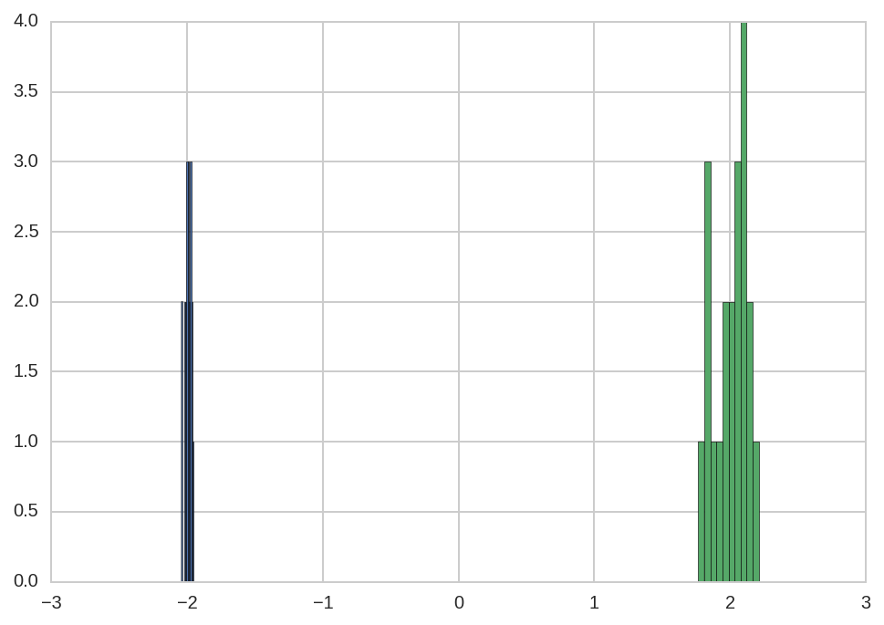
By computing the standard deviation of the peak positions:

In [13]:

dt.query('name == "mu1"')['value'].std()

Out[13]:

0.024538412206652392

In [14]:

dt.query('name == "mu2"')['value'].std()

Out[14]:

0.12309821388429468

we see that the estimation of mu1 as less error than the estimation of mu2.

This difference can be also observed in the histogram of the fitted values:

In [15]:

dt.query('name == "mu1"')['value'].hist()
dt.query('name == "mu2"')['value'].hist(ax=plt.gca());

We can also use pybroom’s tidy_to_dict and dict_to_tidy functions to convert a set of fitted parameters to a dict (and vice-versa):

In [16]:

kwd_params = br.tidy_to_dict(dt.loc[dt['dataset'] == 0])
kwd_params

Out[16]:

{'a2': 0.39327059477457676,
 'ax': 0.39327059477457676,
 'mu1': -1.962722540352284,
 'mu2': 2.1307013636579843,
 'sig1': 0.49895469278155413,
 'sig2': 1.4592545828997032}

In [17]:

br.dict_to_tidy(kwd_params)

Out[17]:

	name	value
0	a2	0.393271
1	ax	0.393271
2	mu1	-1.962723
3	mu2	2.130701
4	sig1	0.498955
5	sig2	1.459255

This conversion is useful to call a python functions passing argument values from a tidy DataFrame.

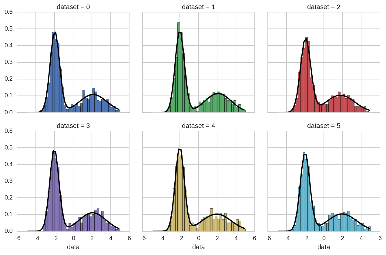
For example, here we use tidy_to_dict to easily plot the model distribution:

In [18]:

bins = np.arange(-5, 5.01, 0.25)
x = bins[:-1] + 0.5*(bins[1] - bins[0])
grid = sns.FacetGrid(ds.query('dataset < 6'), col='dataset', hue='dataset', col_wrap=3)
grid.map(plt.hist, 'data', bins=bins, normed=True);
for i, ax in enumerate(grid.axes):
    kw_pars = br.tidy_to_dict(dt.loc[dt.dataset == i], keys_exclude=['ax'])
    y = model_pdf(x, **kw_pars)
    ax.plot(x, y, lw=2, color='k')

Single-peak model

For the sake of the example we also fit the \(N\) datasets with a single Gaussian distribution:

In [19]:

def model_pdf1(x, mu, sig):
    return normpdf(x, mu, sig)

def log_likelihood_lmfit1(params, x):
    return -np.log(model_pdf1(x, **params.valuesdict())).sum()

In [20]:

params = lmfit.Parameters()
params.add('mu', 0, min=-5, max=5)
params.add('sig', 1, min=1e-6)

Results1 = [lmfit.minimize(log_likelihood_lmfit1, params, args=(di,),
                          nan_policy='omit', method='least_squares')
           for di in d]

In [21]:

dg1 = br.glance(Results)
dg1.drop('message', 1).head()

Out[21]:

	method	num_params	num_data_points	chisqr	redchi	AIC	BIC	num_func_eval	success	key
0	least_squares	6	1	3.136682e+06	-627336.400468	26.958676	14.958676	137	True	0
1	least_squares	6	1	3.060677e+06	-612135.352681	26.934147	14.934147	112	True	1
2	least_squares	6	1	3.260012e+06	-652002.425980	26.997241	14.997241	141	True	2
3	least_squares	6	1	3.096436e+06	-619287.111223	26.945762	14.945762	105	True	3
4	least_squares	6	1	3.097056e+06	-619411.157122	26.945962	14.945962	145	True	4

In [22]:

dt1 = br.tidy(Results1, var_names='dataset')
dt1.query('dataset == 0')

Out[22]:

	name	value	min	max	vary	expr	stderr	init_value	dataset
0	mu	-0.352842	-5.000000	5.000000	True	NaN	NaN	0.00000	0
1	sig	2.233056	0.000001	inf	True	NaN	NaN	1.73205	0

Augment?

Pybroom augment function extracts information that is the same size as the input dataset, for example the array of residuals. In this case, however, we performed a scalar minimization (the log-likelihood function returns a scalar) and therefore the MinimizerResult object does not contain any residual array or other data of the same size as the dataset.

Comparing fit results

We will do instead a comparison of single and two-peaks distribution using the results from the tidy function obtained in the previous section.

We start with the following plot:

In [23]:

dt['model'] = 'twopeaks'
dt1['model'] = 'onepeak'
dt_tot = pd.concat([dt, dt1], ignore_index=True)

In [24]:

bins = np.arange(-5, 5.01, 0.25)
x = bins[:-1] + 0.5*(bins[1] - bins[0])
grid = sns.FacetGrid(ds.query('dataset < 6'), col='dataset', hue='dataset', col_wrap=3)
grid.map(plt.hist, 'data', bins=bins, normed=True);
for i, ax in enumerate(grid.axes):
    kw_pars = br.tidy_to_dict(dt_tot.loc[(dt_tot.dataset == i) & (dt_tot.model == 'onepeak')])
    y1 = model_pdf1(x, **kw_pars)
    li1, = ax.plot(x, y1, lw=2, color='k', alpha=0.5)
    kw_pars = br.tidy_to_dict(dt_tot.loc[(dt_tot.dataset == i) & (dt_tot.model == 'twopeaks')], keys_exclude=['ax'])
    y = model_pdf(x, **kw_pars)
    li, = ax.plot(x, y, lw=2, color='k')
grid.add_legend(legend_data=dict(onepeak=li1, twopeaks=li),
                label_order=['onepeak', 'twopeaks'], title='model');

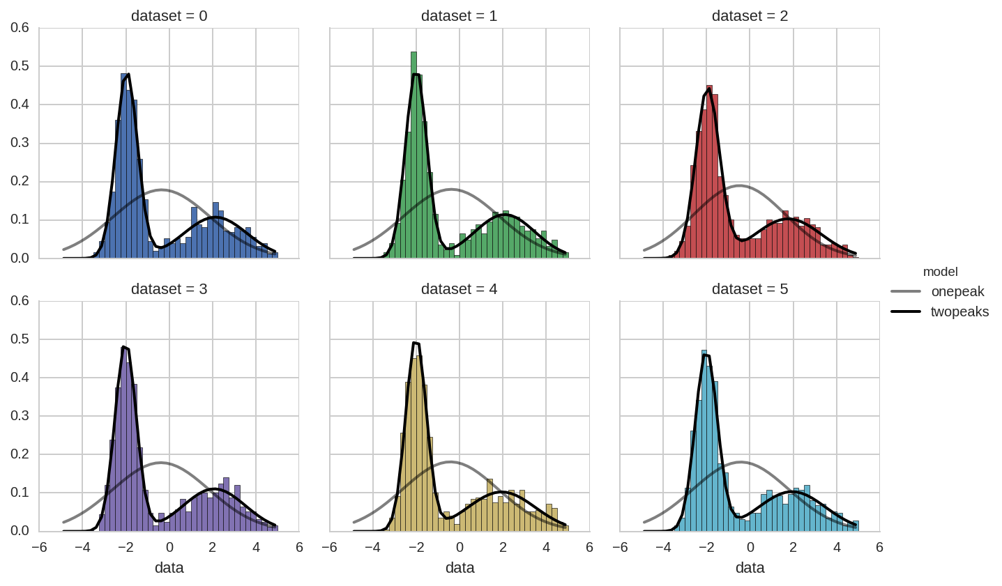
The problem is that FacetGrid only takes one DataFrame as input. In the previous example we provide the DataFrame of “experimental” data (ds) and use the .map method to plot histograms of the different datasets. The fitted distributions, instead, are plotted manually in the for loop.

We can invert the approach, and pass to FacetGrid the DataFrame of fitted parameters (dt_tot), while leaving the simple histogram for manual plotting. In this case we need to write an helper function (_plot) that knows how to plot a distribution given a set of parameter:

In [25]:

def _plot(names, values, x, label=None, color=None):
    df = pd.concat([names, values], axis=1)
    kw_pars = br.tidy_to_dict(df, keys_exclude=['ax'])
    func = model_pdf1 if label == 'onepeak' else model_pdf
    y = func(x, **kw_pars)
    plt.plot(x, y, lw=2, color=color, label=label)

In [26]:

bins = np.arange(-5, 5.01, 0.25)
x = bins[:-1] + 0.5*(bins[1] - bins[0])
grid = sns.FacetGrid(dt_tot.query('dataset < 6'), col='dataset', hue='model', col_wrap=3)
grid.map(_plot, 'name', 'value', x=x)
grid.add_legend()
for i, ax in enumerate(grid.axes):
    ax.hist(ds.query('dataset == %d' % i).data, bins=bins, histtype='stepfilled', normed=True,
            color='gray', alpha=0.5);

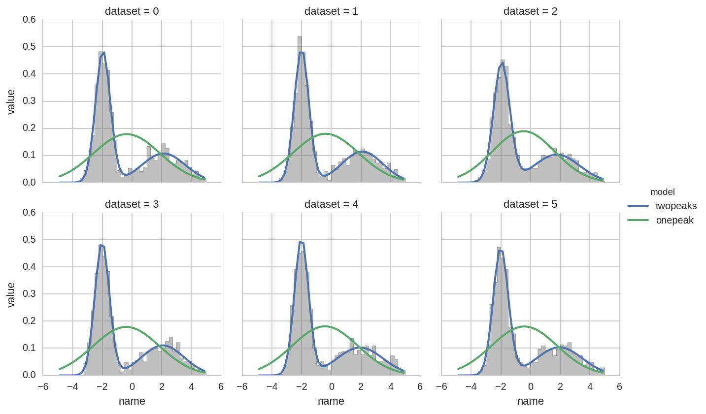
For an even better (i.e. simpler) example of plots of fit results see pybroom-example-multi-datasets.